A machine learning proposal to predict poverty

Una propuesta de aprendizaje automático para predecir la pobreza

Martín Solís-Salazar1, Julio Madrigal-Sanabria2

Solís-Salazar, M; Madrigal-Sanabria, J. A machine learning proposal to predict poverty. Tecnología en Marcha. Vol. 35, No 4. Octubre-Diciembre, 2022. Pág. 84-94.

https://doi.org/10.18845/tm.v35i4.5766

Keywords

Machine Learning; poverty prediction; Proxy Mean Test.

Abstract

Due to the high rate of inclusion and exclusion errors of traditional methods (Proxy Mean Test) used for the identification of households in poverty condition and selection of the social assistance programs beneficiaries, this research analyzed different perspectives to predict households in poverty condition, using a machine learning model based on XGBoost. The models proposed were compared with baseline methods. The data used were taken from the 2019 household survey of Costa Rica. The results showed that at least one of our approaches using XGBoost gave the best balance between inclusion and exclusion errors. The best model to predict poverty and extreme poverty was build using an XGBoost with a classification approach.

Palabras clave

Aprendizaje automático; predicción de la pobreza; Proxy Mean Test.

Resumen

Debido a la alta tasa de errores de inclusión y exclusión de los métodos tradicionales (Proxy Mean Test) utilizados para la identificación de hogares en condición de pobreza y la selección de los beneficiarios de los programas de asistencia social, esta investigación analizó diferentes perspectivas para predecir hogares en condición de pobreza, utilizando un modelo de aprendizaje automático basado en XGBoost. Los modelos propuestos se compararon con métodos de referencia. Los datos utilizados fueron tomados de la encuesta de hogares del 2019 de Costa Rica. Los resultados mostraron que al menos uno de nuestros enfoques utilizando XGBoost dan el mejor balance entre el error de exclusión e inclusión. El mejor modelo se construyó utilizando XGBoost con un enfoque de clasificación.

Introduction

Social assistance programs aiming to help people in poverty conditions require a method to select the beneficiaries. The method must be able to identify people in conditions of poverty and even discriminate between those who are in situations of greater poverty or vulnerability because the resources are limited. The identification of households in poverty is a complex task in developing countries, given the difficulty of accurately measuring the income in informal economies where a high percentage of people has an informal employment [1]

In this context, countries and organizations have developed methods of selecting beneficiaries using proxy variables of income. A common method used in different countries and organizations, such as the US International Development Agency and the World Bank, is the Proxy Mean Test (PMT) [2]. This methodology is based on a regression model that uses a group of income proxy variables collected in surveys to predict the income per capita of the household. Once the model equation has been estimated, the income per capita for each household is computed and a cut-off point is chosen to determine who is in poverty and could be beneficiary of a social assistance program.

In different studies, the suitability of this methodology has been questioned due to the inclusion error rate (IER) and the exclusion error rate (EER) [1, 3, 4, 5]. The inclusion error rate is the proportion of those identified as poor who are not. In this case, the social assistance is protecting households, which are not poor. On the other hand, the exclusion error rate is the proportion of the poor who are not identified as poor. In this case, the social assistance does not attend households, which need support.

According to [1] in Bangladesh, Indonesia, Rwanda and Sri Lanka, the inclusion/exclusion errors are between 44% and 71%, respectively. A study conducted in Sub-Saharan Africa found an inclusion error of 48% and an exclusion error of 81%, where the target was the poorest 20% [6]. This magnitude of error generated by the PMT cause a high incorrect use of economic resources in the fight against poverty.

In this context, our research’s main goal is the analysis of different perspectives to identify households in poverty condition, using a machine-learning model based on XGBoost and the dataset collected through the household survey. The trained models are compared with the traditional methodologies used to create the PMT.

Recent studies on household poverty prediction

Recent studies continue using the typical Multiple Linear Regression to compute the PMT [7, 8]; however, others have used the Quantiles Regression [6]. Some of them predict the income per capita or logarithm of income per capita [9, 10], but also the expenditure per capita is used as dependent variable [5]. There are conclusions drawn to improve the prediction of the classical PMT methodology, for example : a) aggregation of variables that measure characteristics of the home community [6, 9], b) quantile regression at the median [6]; c) the use of the lower confidence interval, instead of the point estimate, when predicting per capita household income [9]; d) selection of variables using new methods, instead of step-by-step regression and manual choice [5].

Due to the weaknesses of the PMT, some recent studies have attempted to model poverty using machine-learning algorithms. One of them was based on data from the Costa Rican Household Survey provided by the Inter-American Development Bank for the model construction that classified households into four groups (Extremely Poor, Moderately Poor, Vulnerable and Non-Vulnerable) using “Random Forest” and also balances the classes with SMOTE [11].

Two other studies attempt to predict the level of household income to determine the degree of poverty [2, 12] with machine learning. In the case of [2], “regression forests”, and “quantile regression forests” were applied to data from the 2005 Bolivian household survey, the 2001 Timor-Leste survey of living standards and the Malawian households 2004-2005. The researchers conclude that the application of cross-validation and stochastic assembly methods produce a gain in the precision of poverty prediction and a reduction in insufficient coverage rates, for which they propose to continue exploring other machine learning methods. On the other hand, [12] only uses machine learning through Random Forest for the selection of the variables that make up the Proxy Mean Square, using data from the 2016 socioeconomic survey of Thailand. Pave and Stender [13] try to predict the poverty rate of Albania, Ethiopia, Malawi, Rwanda, Tanzania, and Uganda for different years using Random Forest as a modeling algorithm and as a mechanism for the selection of variables. Researchers find that this method can improve common practices for predicting poverty.

Method

Data

The data used to train and test the models was the household survey of Costa Rica from 2019, developed by the National Institute of Statistics and Census of Costa Rica (INEC). This survey collected information to estimate the poverty in the country by means of the poverty line method and the multidimensional poverty method. The survey has 34 863 records of members that belong to 11 006 households; however, after deleting some records that had missing information, the final data is composed of 10 923 households. From this total, 6.2% are households in extreme poverty (households with an income per capita less than ₡ 42 117 in the rural area and ₡ 50 618 in the urban area ), 15.8% in poverty (income per capita between ₡ 42 117 and ₡ 86 353 in rural area, and between ₡ 50 618 and ₡112 317 in the urban area), 12.7% are considered vulnerable (income per capita between ₡ 86 353 and ₡ 120 894 in the rural area, and between ₡112 317 and ₡157 243 in the urban area) and 65.3% are non-poverty households. This classification was done based on thresholds in parenthesis. In addition, the household survey of 2018 was used to estimate the weights of an occupation indicator. This will be explained in the next sub section.

Variables

The response variable was poverty classified into four groups: households in extreme poverty, poverty, vulnerability and non-poverty. The classification of households in these groups were defined by INEC according to the income per capita (total income/members ). The response variable was modeled in two ways. First at all, we used as response the income per capita, and from there, the household is classified into one of the four groups according to the threshold calculated by INEC. We named this perspective as indirect estimation. Second, poverty was modeled directly as a classification case.

The variables used to predict the poverty are related with the conditions of the house, services of the household, ownership of assets, variables of the poverty multidimensional method and sociodemographic characteristics of household members. The predictor’s variables are indicated briefly in table 1. Next, we will explain two important indicators that we created and are not included in other studies on poverty prediction as far as we know.

Occupation indicators

We assigned a weight to 50 groups of occupations of the household members according to the relevance of the occupation in terms of salary received. These fifty occupations are determined by the combination of three variables: a) condition of the employee (private sector employee, public sector or NGO’s employee, household employee, self-employed with employees, self-employed without employees), b) category of job (director, high or executive manager, professional and intellectual jobs, technicians, administrative support, service workers and shop sellers, farmers, agricultural workers, forestry and fishing workers, machine operators and agents (mechanical, art, electricity and other machines, facilities operator, assemblers, elementary occupations such as informal sellers, unskilled farmer workers, cleaning assistants, and others), c) pensioners and people who earn money through personal investments according to their level of education (without formal education, primary education, secondary education and university education)

The weight assigned is the mean salary of each group according to household survey of 2018. Once the weights of each occupation were calculated, two indicators were computed. The first one is the occupation weight of the household head, and the second is the mean occupation weight of the total household members. This last one was computed dividing the sum of the indicator weights by the total members of the household. The member who didn’t have a remunerated job, or wasn’t a pensioner or a rentier, had a value of zero.

Appliance indicator

It is the number of appliances of the household. The maximum score was 17. It includes basic appliances such as refrigerator and more fancy devices such as computers, tablets, and cars.

Table 1. Variables used.

Category	Variables
Conditions of the house	Wall condition, floor material, floor condition, roof condition, roof material, wall material, paid TV, have a toilet, kind of toilet, number of bedrooms, squared number of bedrooms, has ceiling, overcrowding in bedrooms, number of rooms, rooms per person, overcrowding in rooms, size of the house, meters of construction per member, number of bathrooms, owner of the house, rent payment.
Services of the house	Water source, water supply, has Internet, kitchen energy source, has electricity, private electricity plant, service of garbage management.
Ownership of assets	Has a car, appliance indicator, cars per person older than 18, has computer, cell phones per person older than 12, computers per person older than 12, tablets per person older than 12, number of cars, number of computers, number of cell phones, number of tablets, have cell phone in the house.
Multidimensional poverty variables	Twenty indicators of poverty multidimensional method
Sociodemographic characteristics	Number of members, sex of the head, age of the head, squared age of the head, non-formal education, civil status of head, dependency rate, squared dependency rate, disability of head, education years of head, squared education years of head, rate of members that have non-formal education tittle, number of elderly, number of children, rate of members that received economical support help, mean education years of adults, mean education years of all members, mean of occupation indicator, occupation indicator of the head, instruction level, number of members with years behind the school, occupation of the head, position of occupation of the head, job sector of the head, men less than 12, men older than 12, total men, women less than 12, women older than 12, total women, members less than 12, members older than 12, members less than 12, sex of the head, squared members less than 18, region of residence, area of residence (urban vs rural)

Procedure

Algorithms

Our proposals for poverty prediction were based XGBoost. XGBoost is widely used by data scientists [14] to improve the state of the art in regression and classification problems. It is an ensemble algorithm of trees where each tree considers the error of the previous one. It has an objective function composed of a loss function that measures the difference between predicted and real values, and a regularization part that penalizes the tree’s complexity

With XGBoost, the poverty was modeled in three ways: a) indirectly, as was explained; b) directly, with the prediction of the four categories of poverty (multiclass classification); c) directly, building a model for each category of poverty. This last perspective implies moving from a multiclass classification approach to a binary classification approach.

Our proposals were compare with the next baseline models: a) Multiple Linear Regression to predict the income per capita of households, and assign later the category of poverty with the thresholds established by the National Institute of Statistics and Census of Costa Rica; b) Multiple Linear Regression, using only 40% of the households with the minimum income per capita, as was suggested by [9]; c) SMOTE+Random Forest as was applied by [11], d) Quantile regression forest, as was applied by [2].

It is convenient to develop a model with the few amount of variables as possible, because the users of the model will require the collection of less information to classify the household. To that end, we also used the next Feature Reduction algorithms: A) Recursive Feature Elimination using Random Forest (RF-RFE). First proposed by [15]. A model with Random Forest is trained. Next, a ranking of the feature importance was computed based on their contribution to the prediction. Finally, the least important features were removed. B) Minimum Redundancy Maximum Relevance (mRMR). First proposed by [16].This algorithm operates minimizing redundancy of the features while maximizing relevancy of the attributes selected based on mutual information. C) Relief. According to [17] the idea behind this proposal is that relevant features are those whose values can be distinguished among closer instances.

Preprocessing and data division

In this phase the variables were computed and normalized between 0 and 1, the records with missing information were deleted, and the data with the 10 923 households of 2019 was randomly divided into two parts: 75% for training and tuning and 25% for validation.

In the training phase, a 3-fold cross-validation approach was used to define the parameters values of the algorithm (tuning process). Therefore, the training set (75% of our original dataset) was divided into training and testing 3 times for each parameter combination to select the best model. This procedure consists of taking 2/3 of the sample to calibrate the algorithm with specific parameters and 1/3 to predict the observations. This is replicated three times (3 non-overlapping training and testing sets). At the end of the process, the predictions results of these three replications were averaged, for each combination of parameters. In total, 1000 different combinations of parameters randomly generated were tested, but only the best was chosen, according to the minimization of the loss function, that were the squared mean in the XGBoost-indirect (regression) and the multiclass logloss (multiclass cross entropy) and binary logloss (binary cross entropy). The parameters of XGB Boost used to be evaluated are: max depth, min_child_ weight, gamma, colsample_bytree, subsampled.

The predictive capacity of the algorithms was evaluated with different measures, using the validation data and the measures shown below.

1.IER=Inclusion rate for extreme poverty, cumulative poverty and cumulative vulnerability. It is the proportion of households included incorrectly

2.EER=Exclusion rate for extreme poverty, cumulative poverty and cumulative vulnerability. Proportion of households excluded incorrectly

3.F macro score of extreme poverty, poverty and vulnerability. In this case, the F score is calculated without the accumulation of the poverty categories. For example, in the previous case, vulnerability includes extreme poverty, poverty and vulnerability, while this case only considers the punctual category of vulnerability.

4.Total accuracy.

5.R-squared for the models where the prediction variable is the income per capita.

Results

Table 2 shows the performance metrics of baseline models and our machine learning perspectives. The results suggest that for Extreme Poverty and Poverty, at least one of the baseline models showed a better IER or EER, but not both, and when one of these two metrics is better, another is considerably worst. Therefore, the mean of both kinds of errors is better in at least one of our proposals. It is desirable a model with similar IER and EER because both have negative implications, and our proposal XGBoost direct showed the best balance of these metrics. On the other hand, in vulnerability the best option was XGBoost direct_ind, but with similar results to the baseline QRF. In regard to the global metrics, XGBoost direct show the best F macro and accuracy, meanwhile XGBoost indirect has the best R^2. Finally, the comparison of our models indicates that it is better to build a model based on a classification perspective (XGBoost direct or XGBoost direct_ind) instead of a regression perspective (XGBoost indirect).

Table 2. Performance measures of the models based on validation sample.

Models	Extreme			Poverty			Vulnerability			Global
	IER	EER	Mean	IER	EER	Mean	IER	EER	Mean	F macro	Acc	R^2
MLR	69%	72%	71%	34%	49%	41%	18%	37%	28%	44%	68%	57%
MLR 40% [9]	33%	92%	63%	47%	22%	34%	54%	3%	28%	34%	41%	43%
SMOTE+RF [11]	56%	63%	59%	43%	25%	34%	33%	18%	25%	50%	66%	-
QRF [2]	31%	87%	59%	23%	46%	35%	21%	28%	24%	48%	71%	58%
XGBoost direct	40%	66%	53%	27%	32%	29%	14%	39%	27%	52%	74%	-
XGBoost direct_ind	41%	72%	56%	27%	38%	32%	20%	24%	22%	-	-	-
XGBoost indirect	46%	85%	65%	24%	54%	39%	17%	36%	27%	45%	70%	62%

MLR=Multiple Linear Regression; MLR 40%= MLR trained with the 40% of the poor households; SMOTE+RF =Random Forest + SMOTE; QRF =Quantile Regression Forest; XGBoost-direct= XGBoost for multiclass classification; XGBoost-direct_ind = XGBoost for classification using dummy output; XGBoost-indirect= XGBoost for regression. In black the best result.

Figure 1 shows three graphs to explain the most influential variables based on the shape method (Lundberg, & Lee, 2016) in the identification of extreme poverty, poverty and vulnerability, using the validation sample and XGBoost direct. This method computes Shapley values from the coalitional game theory. The Shapley values indicate to which level each feature in the XGBoost-direct contributes, either positively or negatively, to each prediction. The vertical axes show the degree of importance of the five most important variables. The degree of importance is the mean of Shapley values per feature across de data test records. The color describes the value of each point. Blacker dots means higher values, while whiter points means the contrary. The horizontal axis indicate whether each value is associated with a high or low value prediction based on Shapley values. In the three graphs, we can see that the most important variable so far is the mean of the occupation indicator. Neither of the graphs shows a clear tendency of how color influences the classification, mainly because this variable tends to have low values in the range between 0 and 1 (all the variables were standardized in this range), and it is difficult to distinguish between light gray colors. In addition, the appliance indicator was among the most important, specifically in the prediction of extreme poverty and vulnerability. In the graph, whiter colors are associated with the condition of extreme poverty and poverty, therefore in the case of appliance indicator, less appliances mean more poverty (a negative correlation with the probability of poverty).

In addition, there are two indicators of multidimensional poverty between the most significant variables. The first one is the condition of at least one person between 18 and 24 years old without secondary education. This condition influences the probability of being classified as extreme poverty, because the black points that represent the presence of this condition have positive Shapley values, which means that this condition is associated with higher probability of extreme poverty. The second one is the condition of at least one person without health care insurance. This condition tends to be associated with poverty. Other important variables associated with poverty are the proportion of members that receive economic help from governmental institutions; the mean number of education years of all members in the household and the mean number of education years of the adult members.

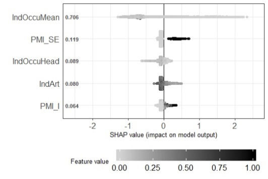
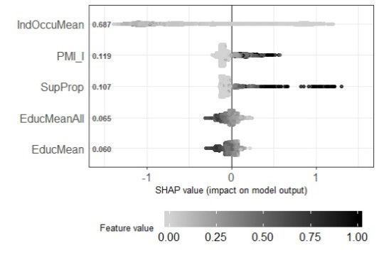
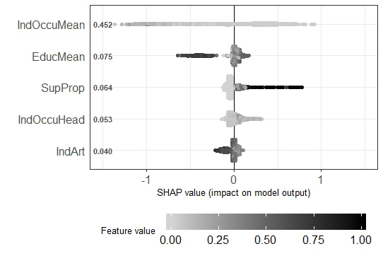
Figure 1. Shapley values from the five most influential variables in the prediction of poverty. IndOccuMean= mean of occupation indicator of the total household members; PMI_SE = Poverty Multidimentional Indicator (at least one person between 18 and 24 years old without secondary education); IndOccuHead=Indicator of occupation of the head at the household; IndArt=Appliance Indicator; IPM_S1F= Poverty Multidimentional Indicator (at least one person without health care insurance); SupProp= Proportion of members that receive economic help from institutions; EducMeanAll= Average years of schooling of all members in the household; EduMean= Average years of schooling of adults.

In order to build a model with fewer variables, we applied five feature selection methods previously to the training of the XGBoost-direct. table 3 shows the performance metrics of the XGBoost-direct after feature selection. With the method Recursive Feature a wrap of variables were evaluated, and the optimal number was 30. Meanwhile, with the methods Relief and Minimum Redundancy Maximum Relevance we proved different numbers of variables, specifically, a simplified model with 15, 35 and 55 variables. All the models showed worst performance than the model with all the variables, although in some cases gave close results to original model in Poverty and Vulnerability, as it is mRMR55 or RF with 30 variables. The selection of 15 variables with RF generates the best simple model, but the IER and EER increase 3.7 and 4.8 percentage points respectively in poverty. These increments cause more resources to be allocated incorrectly; however, it is the decision makers who must decide between a more complex model that requires collecting more information and a simpler model that can generates a slightly larger error. In extreme poverty, the variable reduction affects more the model performance when it has less than 55 variables.

Table 3. Performance measures of XGBoost-direct (classification) with Feature Selection.

Models	Extreme poverty			Poverty			Vulnerability			Global
	IER	EER	Mean	IER	EER	Mean	IER	EER	Mean	Fmacro	Acc
RF	48%	73%	61%	31%	33%	32%	15%	40%	28%	49%	73%
RE15	50%	76%	63%	31%	37%	34%	15%	43%	29%	47%	72%
RE35	49%	73%	61%	31%	34%	33%	15%	40%	28%	49%	73%
RE55	42%	71%	57%	31%	36%	34%	14%	41%	28%	49%	73%
mRMR15	36%	81%	59%	33%	37%	35%	15%	44%	30%	45%	72%
mRMR35	34%	73%	54%	31%	36%	34%	14%	43%	29%	49%	73%
mRMR55	41%	66%	54%	30%	32%	31%	14%	40%	27%	51%	74%

RF=Recursive Feature Elimination with Random Forest; RE= Relief; HC= mRMR =Minimum Redundancy Maximum Relevance feature selection.

Conclusions

This paper compares traditional methods to predict poverty with a machine learning approach based on XGBoost. The results showed that baseline methods were surpassed by at least one of the XGBoost perspectives, considering the balance between IER and EER in extreme poverty, poverty and, vulnerability. Our best model for poverty and extreme poverty was XGBoost using the multiclass classification approach. In addition, we found that the classification approach gave better results than the regression approach.

The performance of our models appears suitable when compared with some results of the traditional methods applied in other recent studies. For example, the R squared of the XGBoost indirect was of 0.62 in tests, and it is uncommon to find an R squared higher than 0.60 [5, 6, 7] to predict the income per capita. Moreover, the exclusion and inclusion error rate of any XGBoost in our study is better than in other studies that have targeted a percentile around 20% of poor households [6, 8]. On the other hand, the Inter-American Development Bank did a competition in Kaggle to predict poverty with data of the household survey of Costa Rica, similar to us, and the winner model obtained a F macro of 0.44 (https://www.kaggle.com/c/costa-rican-household-poverty-prediction/overview), while our best model obtained a F macro of 0.517. All these comparisons must be taken with care, because it is clear that neither the data used for training and testing were the same, nor the result of Kaggle’s winner model.

Finally, we applied Feature Selection algorithms to reduce the number of variables, in order to require the collection of less information to classify the household. Our results showed that it is possible to reduce the number of variables to 15, increasing in 3.7 and 4.8 percentage points the IER and EER for poverty prediction. However, in extreme poverty the variable reduction affects more the model performance when it is fewer than 55 variables.

Future lines of research

The surveys could have records with biases in the variables. This bias could cause noise that influences the training process, and generates misclassification. For this reason, a future area of work is identification of the biases in the household surveys using machine learning. If it is possible to exclude the record with biases, training to predict poverty could improve and at the same time correct the classification.

An option that could be explored is the use of images of houses to classify the households as poor and non-poor. Some studies have shown the power of Convolutional Neuronal Network trained with images of houses for the prediction of outputs as the house price [18] and Architectural Style [19]. Hence, in the same way, the CNN could have power to predict poverty using as input internal and external images of houses, and as output, the income per capita or the classification of the household according to poverty degree estimated through surveys. When the institutions conduct surveys to collect the variables of poverty estimation in a country, they can take pictures of houses, following a protocol of application.

Another option is to use the photos of houses and the CNN to extract features that can be the input, together with other variables such as those used in this study, for poverty prediction. In addition, the variables provided by surveys could be combined with features extracted from satellite images of the areas where the households interviewed are located. Some studies have used satellite images to predict variables associated with the income of areas[20, 21]; consumption expenditures of areas [22] and poverty rate of regions [23].

Referencias

[1] S , Kidd and E, Wylde, E, “Targeting the Poorest: An Assessment of the Proxy Means Test Methodology” Technical report, AusAID, Washington, DC, 2011

[2] L, McBride and A, Nichols, “Retooling poverty targeting using out-of-sample validation and machine learning”, The World Bank Economic Review, vol. 32, no. 3, pp. 531-550, 2018.

[3] D, Budlender “Considerations in Using Proxy Means Tests In Eastern Caribbean States”., St.Lucia, 2016.

Available:https://pdfs.semanticscholar.org/efab/96de659b7208f41382341cf206ac25 9838c.pdf. [Accessed: March. 18, 2020].

[4] F, Delgado-Jiménez, “Efectividad en la selección de beneficiarios de los programas avancemos y bienestar familiar”, Economía y Sociedad, vol. 22, no. 52, pp. 1-24, 2017

[5] A, Bah, “Finding the Best Indicators to Identify the Poor”,Working Paper 01-2013, Jakarta, Indonesia: National Team for the Acceleration of Poverty Reduction (TNP2K), 2013

[6] C ,Brown. M Ravallion and D, Van de Walle, “A Poor Means Test? Econometric Targeting in Africa”, Working Paper 22919, Massachusetts, EEUU: National Bureau of Economic Research, 2016.

[7] S, Kidd. B. Gelders and D, Bailey-Athias, “Exclusion by design: an assessment of the effectiveness of the proxy means test poverty targeting mechanism”, ESS Working Paper No.56, Geneva: International Labour Office, 2017

[8] S, Ashwini, et al, “A Proxy Means Test for Sri Lanka,. Working Paper 8605, 2018

[9] D. S Mapa. & , M.L.F, Albis, “New Proxy means test (PMT) models: improving targeting of the poor for social protection”. In 12th National Convention on Statistics, Manila, Philippines, 2013.

[10] R. K , Dewi and A, Suryahadi, “The implications of poverty dynamics for targeting the poor: simulations using Indonesian data”, Working paper, SMERU Research Institute, Indonesia, 2014

[11] J, Hussein. O, Nazih, “Poverty level characterization via feature selection and machine learning”, In 27th Signal Processing and Communications Applications Conference (SIU), Siva, Turkey, 2019.

[12] M, Pisacha, “Better Model Selection for poverty targeting through Machine Learning: A case Study in Thailand”, M.S. thesis, Thammasat University, Thailand, 2017

[13] T, Pave and N, Stender, “Is random forest a superior methodology for predicting poverty? an empirical assessment”. Poverty & Public Policy, vol. 9, no. 1, pp. 118-133, 2017

[14] T, Chen and C Guestrin, “Xgboost: A scalable tree boosting system”, In Proceedings of the 22nd ACM SIGKDD Conference on Knowledge Discovery and Data Mining, EEUU, San Francisco, CA, USA, 13 August 2016.

[15] Guyon, et al, “Gene selection for cancer classification using support vector machines”. Machine learning, vol 46, no.1, pp. 389-422, 2002

[16] H. Peng , F. Long , C. Ding, “Feature selection based on mutual information: cri- teria of max-dependency, max-relevance, and min-redundancy”, IEEE Trans. Pattern Anal. Mach. Intell. Vol. 27, pp. 1226–1238, 2005

[17] S. García. J, Luengo. F. Herrera. “Tutorial on practical tips of the most influential data preprocessing algorithms in data mining”, Knowledge-Based Systems, vol. 98, pp. 1-29, 2016

[18] O, Poursaeed. T, Matera, T. S, Belongie, “Vision-based real estate price estimation”. Machine Vision and Applications, vol. 29, no. 4, pp. 667-676, 2018

[19] Y. Yoshimura et al, “Deep learning architect: classification for architectural design through the eye of artificial intelligence”. In International Conference on Computers in Urban Planning and Urban Management (pp. 249-265). Springer, Cham, 2019

[20] R, Ngestrini, “Predicting Poverty of a Region from Satellite Imagery using CNNs”, M.S. thesis, Utrecht University, Utrecht, 2019

[21] S.M, Pandey. T, Agarwal. N.C, Krishnan, “Multi-task deep learning for predicting poverty from satellite images”, In Thirty-Second AAAI Conference on Artificial Intelligence, New Orleans, USA, 2018

[22] N. Jean, et al, “Combining satellite imagery and machine learning to predict poverty”. Science, vol. 353, pp. 790-794, 2016

[23] V.H, Maluleke. S, Er. Q. R Williams, “Estimating poverty using aerial images: South African application”. Data Science and Applications, vol.1, no. 1, pp. 29-36, 2018.

---